Key Messages
- Effectiveness is objective-dependent. A control can operate as designed without achieving its intended objective.
- Control design is multidimensional. Effectiveness depends on whether the design addresses the relevant dimensions of the objective.
- Population quality matters. Testing can only provide reliable evidence when the underlying population is complete, relevant and representative.
- Operating effectiveness is not enough. A control may operate consistently while the available observations remain insufficient to demonstrate the intended outcome.
- Conclusions must be proportionate to evidence. The strength of a conclusion depends on the objective, the quality of the evidence and the amount of information available.
A control can operate exactly as designed and still fail to achieve its intended objective.
Conversely, an adverse outcome does not necessarily mean that a control has failed.
I find this distinction particularly interesting when looking at quantitative processes. We can define a procedure, implement it correctly and demonstrate that it operates as intended. Yet we may still lack the evidence needed to establish that it achieves the objective for which it was designed.
P&L attribution provides a useful example. Depending on its purpose, the same process can explain historical results, diagnose weaknesses in a risk model, or assess whether model-guided decisions generate profitable outcomes.
The process may look similar. The claim we want to establish is not.
Start with a simple control
Consider a straightforward control in an insurance company:
Every supplier payment above CHF 10,000 must receive a second approval before it is released.
This is a form of segregation of duties. Its objective is to reduce the risk of unauthorized or inappropriate payments.
Two questions follow.
Design effectiveness: Would the control address the underlying risk if it were performed as intended?
That requires us to examine the threshold, the independence of the second approver, the timing of the approval and the treatment of exceptions.
Could payments be split to avoid the threshold? Are all relevant payment channels covered? Can the second approver challenge the transaction independently, or does that person simply rely on the first approver?
Operating effectiveness: Was the control actually performed as required?
That requires evidence that all relevant payments were identified, that the second approval was obtained before release, and that the procedure was followed consistently.
A documented approval may demonstrate compliance with the procedure without proving that the control is well designed. Equally, a well-designed control may not operate consistently in practice.
Testing introduces another challenge: we need a complete population of payments to which the control applies. If transactions are missing, or the sample excludes unusual transactions and exceptions, the evidence may give a misleading impression of effectiveness.
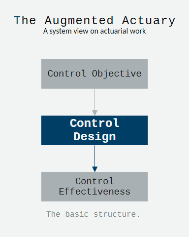
The basic structure is straightforward:
Define the objective → design the control → test its operation → determine what the evidence supports.
The difficulty is that, outside deterministic controls, neither the objective nor the evidence requirements are always so clear-cut.
P&L attribution has different objectives
Under Solvency II, Article 123 requires insurers and reinsurers to review, at least annually, the causes and sources of profits and losses for each major business unit. The undertaking must demonstrate how the risk categorisation used in its internal model explains those causes and sources. Article 240 of Delegated Regulation (EU) 2015/35 further addresses profit and loss attribution.
But P&L attribution can serve purposes beyond regulatory compliance.
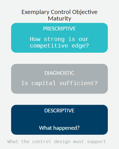
I distinguish three objectives.
| Objective | Key question | What the design must support |
|---|---|---|
| Descriptive | What happened? | Consistent P&L definitions, reconciliation, traceability and attribution |
| Diagnostic | Is the capital model sufficient? | Granularity to identify risk drivers, investigate tail outcomes, assess dependencies and detect model weaknesses |
| Prescriptive | How strong is our competitive edge? | Explicit hypotheses, appropriate observations, statistical power, out-of-sample evaluation and evidence of repeatable economic value |
Descriptive attribution: What happened?
The control must ensure that P&L is defined consistently, reconciled to relevant financial results and attributed to the appropriate business units and risk categories.
The emphasis is on completeness, traceability and consistency.
Diagnostic attribution: Is the capital model sufficient?
Aggregate P&L may conceal offsetting errors across risk categories. A result close to expectation may coexist with weaknesses in the model’s representation of dependencies. An adverse outcome may be consistent with the modelled distribution—or may reveal an inadequate assumption.
The control therefore needs appropriate granularity, sensitivity analysis, backtesting and investigation of material deviations. A design sufficient for reporting may not be sufficient for diagnosis.
Prescriptive attribution: How strong is our competitive edge?
Here the objective changes. Explaining historical outcomes is not enough. We want to know whether the model identifies opportunities that generate a genuine, repeatable economic advantage.
That requires a test designed around a specific claim about future performance. The observation unit, evaluation period, success criterion and statistical methodology must all be appropriate to that claim.
A process can be effective for descriptive attribution while being insufficient for prescriptive analysis. That does not necessarily mean the process has failed. Its design may simply not have been intended to establish profitability.
The effectiveness of a control is therefore relative to its objective.
From estimated edge to statistical evidence
In my SoccerSim Insurance Lab, I use a simplified betting strategy to make this challenge tangible.
Consider a market with three possible outcomes. A bookmaker’s prices incorporate an overround, while a model attempts to identify opportunities whose expected return is positive after the relevant costs.
Assume a 3% bookmaker overround and equal decimal odds across the three outcomes:
\[o=\frac{3}{1.03}\approx2.9126\]For a unit stake on one selected outcome, the net payoff is approximately +1.9126 units if the bet wins and −1 unit if it loses.
Suppose the strategy has a true expected net return of +10% per unit staked. This is an illustrative assumption, not evidence that the strategy has already demonstrated that return.
At these odds, the win probability required to achieve that expected return is:
\[p=\frac{1.10}{2.9126}\approx37.77\%\]The bookmaker’s overround determines the offered odds. The strategy’s edge must be demonstrated separately.
Quantify the uncertainty
For a unit stake, the variance of the net return is:
\[\operatorname{Var}(X) =p(o-1)^2+(1-p)(-1)^2-\mu^2\]With an assumed expected net ROI of 10%, this gives approximately:
\[\operatorname{Var}(X)\approx1.994\]and a standard deviation of:
\[\sigma_X\approx1.412\]The standard deviation is substantial relative to the expected return. Individual outcomes are noisy, even when the assumed edge is genuine.
That is the central problem: a positive expected return does not guarantee a positive result over a short observation period.
How much evidence is enough?
Let \(\(X_i\)\) be the net return on the (i)-th unit stake. We want to test whether the expected return differs from zero:
\[H_0:\mu=0 \qquad\text{versus}\qquad H_1:\mu\ne0\]For illustration, assume:
- A two-sided confidence level of 90%, corresponding to a 10% significance level.
- Statistical power of 80%.
- A true expected net ROI of 10%.
- Independent observations and a stable payoff distribution.
A normal-approximation planning formula that allows for different standard deviations under the null and alternative is:
\[n\approx \left( \frac{z_{0.95}\sigma_0+ z_{0.80}\sigma_1}{\delta} \right)^2\]Here, $\delta$ is the assumed true ROI, $\sigma_0$ is the standard deviation under the null hypothesis, and $\sigma_1$ is the standard deviation under the assumed alternative.
Using $\sigma_0 \approx 1.383$, $\sigma_1 \approx 1.412$, $z_{0.95} \approx 1.645$ and $z_{0.80} \approx 0.842$:
\[n\approx \left( \frac{1.645(1.383)+0.842(1.412)}{0.10} \right)^2 \approx1{,}199\]The result is approximately 1,200 independent bet observations.
Translate observations into seasons
Suppose the strategy identifies seven to eight bets per matchday, with equal stakes. Normalise the total amount staked across the selected bets to 100%.
- Eight bets each represent 12.5% of total stakes.
- Seven bets each represent approximately 14.29% of total stakes.
- At a 10% expected net ROI, expected portfolio profit is 10% of total stakes.
Assume a league season contains 34 matchdays.
| Measure | Illustrative result |
|---|---|
| Selected bets per matchday | 7–8 |
| Bets per season | 238–272 |
| Required independent bets | Approximately 1,200 |
| Required matchdays | Approximately 150–172 |
| Equivalent seasons | Approximately 4.4–5.1 |
Under these assumptions, one season supplies 238–272 raw bet observations, compared with approximately 1,200 independent observations required for 80% power.
One season can still be informative. It can reveal a promising signal, expose model weaknesses or indicate poor performance. It may not, however, provide sufficient evidence to establish a 10% edge with the specified confidence and power.
The point is not that every profitability test requires five seasons. The result depends on the effect size, variability, dependence and test specification.
The observation unit matters
There is a subtle but important distinction between the number of records and the number of independent observations.
If the hypothesis concerns individual-bet expected ROI, individual bets may be the relevant observation unit, provided their dependence is appropriately addressed.
If the hypothesis concerns aggregate matchday profitability, each matchday’s portfolio P&L may instead be the observation unit.
Aggregating bets does not create additional information. The mean, variance and sample size must all refer to the same observation unit.
The same issue arises in insurance. A portfolio may contain thousands of policies or claims, but these observations can share exposure to common economic conditions, catastrophe events, underwriting changes or model assumptions.
The observation unit must follow the hypothesis—not simply the number of records in the data.
What the calculation does and does not establish
The sample-size calculation assumes a stable payoff distribution and independent observations. In practice, both the mean and standard deviation are estimated, and dependence may reduce the effective amount of information. We may also need to assess the parameters at portfolio level.
The result is sensitive to the size of the true effect. A smaller edge or higher variability requires more observations. Heavy-tailed outcomes, rare events and changing conditions can make a simple normal approximation unreliable.
Statistical power is the probability that a specified test detects an effect of a given size under its assumptions. It is not the probability that the model is correct, nor the probability that the strategy is profitable.
Nor can a large number of Monte Carlo simulations substitute for independent real-world evidence. Simulations can improve the numerical precision of a model-implied distribution, but they do not prove that the model’s assumptions are correct or that its estimated edge will persist in practice.
Finally, an estimated ROI from the same data used to select or tune a strategy is not independent validation. Repeatedly testing variants and reporting only the best-performing strategy introduces selection bias. Out-of-sample evaluation and a prespecified test are essential when the intended conclusion concerns repeatable future profitability.
What this reveals about control design and testing
The supplier payment control and P&L profitability example illustrate the same underlying challenges.
The control objective can be subjective or multidimensional.
A deterministic control can often be assessed against an explicit rule. But objectives such as adequate risk representation, model effectiveness or profitable decision-making require judgement about what constitutes success.
If the objective is vague, the control design and test criteria will be vague as well.
Control design has multiple dimensions.
Scope, thresholds, risk categorisation, assumptions, dependencies, observation units and evaluation criteria all determine what the control can establish.
A control may be well designed for regulatory reporting but inadequate for detecting model weaknesses. A methodology may explain historical results but be unsuitable for testing predictive profitability.
Testing depends on the quality of the population and observations.
Missing transactions, incomplete data, unrepresentative samples and poorly defined observation units can undermine otherwise correct procedures.
In quantitative testing, dependence and variability introduce additional constraints. Hundreds of records may provide substantially less independent information than their count suggests.
Operating effectiveness does not guarantee sufficient evidence.
A test can be executed correctly and still be inconclusive. In the profitability example, the assumed edge is positive, but one season supplies fewer observations than the illustrative calculation requires.
The issue is not necessarily a failure of execution. It is a limitation of the evidence available to support the conclusion.
Conclusions must be proportionate to the evidence.
No observed exceptions does not prove that a control never fails. An explained historical result does not prove predictive power. A statistically significant result does not automatically establish economic materiality or repeatability.
A defensible control framework makes these boundaries explicit and avoids claiming more than the evidence supports.
Conclusion
P&L attribution demonstrates why control design and testing are inseparable from the objective being pursued.
At the descriptive level, the control must provide complete, consistent and traceable explanations of historical P&L. At the diagnostic level, it must reveal the risk drivers and model weaknesses that aggregate results can conceal. At the prescriptive level, it must support a test that distinguishes a genuine economic advantage from random variation.
The requirements become more demanding because the claim itself becomes more demanding. Design choices determine what can be established, and the available evidence determines how confidently it can be established.
The central discipline is straightforward:
Define the objective. Design the control for that objective. Test it against an appropriate population using a defensible methodology. Draw only the conclusions the evidence supports.
That is the broader lesson of P&L attribution for control assurance: effectiveness is not an absolute property of a procedure. It is a conclusion about a defined objective, a specific design and the strength of the evidence gathered through testing.
Regulatory references: Solvency II Directive, Article 123 (Profit and loss attribution); Solvency II Delegated Regulation (EU) 2015/35, Article 240 (Profit and loss attribution).
The quantitative example is illustrative. The assumed mean and standard deviation are not empirical estimates or prescribed regulatory thresholds.
Tags: risk, insurance, model-risk, control-effectiveness, quantitative-testing